Examples
Tikhonov reconstructions for a bi-Maxwellian distribution
In this example, we will reconstruct the bi-Maxwellian fast-ion velocity distribution using the 0th order and 1st order
regularisation matrix. This example is identical to demos/biMax_recon.m.
%% Bi-Maxwellian Reconstruction Example
% This is a demo of a velocity-tomography example, where
% we reconstruct the bi-Maxwellian fast-ion velocity distribution
% with the 0th and 1st order Tikhonov formulation.

clear, clc, close all

[A, b, x, L, ginfo] = biMax();
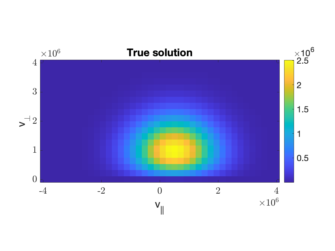
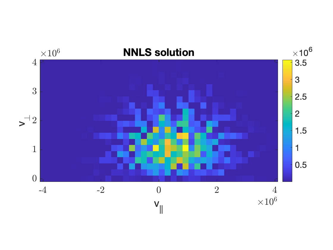
Now using the function showDistribution we can display the true solution and the least-squares solution, which we get by setting
\(\alpha = 0\).
%Display the true solution
figure
showDistribution(x,ginfo); title('True solution')
%Display nonnegative least-squares solution
figure
showDistribution(TikhNN(A,b,0,[]),ginfo); title('NNLS solution')
%0th order Tikhonov.
disp('Solving 0th order Tikhonov.')
alpha0 = logspace(-15,-8,20);
xalpha0 = TikhNN(A, b, alpha0, []);
[ralpha0, idx0] = relerr(x, xalpha0);
fprintf('Optimal solution: alpha = %.2e, r(alpha) = %.5f\n',alpha0(idx0),ralpha0(idx0))

figure;
semilogx(alpha0, ralpha0); xlabel('\alpha'); ylabel('Relative error')
hold on
plot(alpha0(idx0),ralpha0(idx0), '.', 'MarkerSize',15); ylim([0 max(ralpha0)])
title('Relative error, 0th order Tikhonov')

figure
showDistribution(xalpha0(:,idx0),ginfo); title('Optimal 0th order Tikhonov solution')
For the 0th order Tikhonov, this gives us the following plot of the relative error as a funciton of the regularisation parameter \(\alpha\).
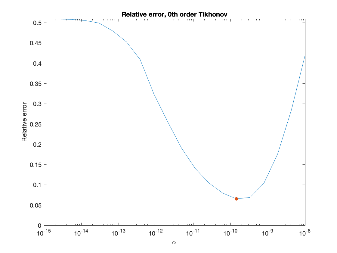
with the optimal regularisation parameter \(\alpha = 1.44\cdot10^{-10}\) and minimum relative error \(0.06522\). Once again, we can use showDistribution
to display the optimal 0th order solution.

For the 1st order Tikhonov, we pass the regularisation matrix L to TikhNN in order to penalize large norms in the 1st order derivative.
%1st order Tikhonov.
disp('Solving 1st order Tikhonov.')
alpha1 = logspace(-4,4,20);
xalpha1 = TikhNN(A, b, alpha1, L);
[ralpha1, idx1] = relerr(x, xalpha1);
fprintf('Optimal solution: alpha = %.2e, r(alpha) = %.5f\n',alpha1(idx1),ralpha1(idx1))
figure;
semilogx(alpha1, ralpha1); xlabel('\alpha'); ylabel('Relative error')
hold on
plot(alpha1(idx1),ralpha1(idx1), '.', 'MarkerSize',15); ylim([0 max(ralpha1)])
title('Relative error, 1st order Tikhonov')
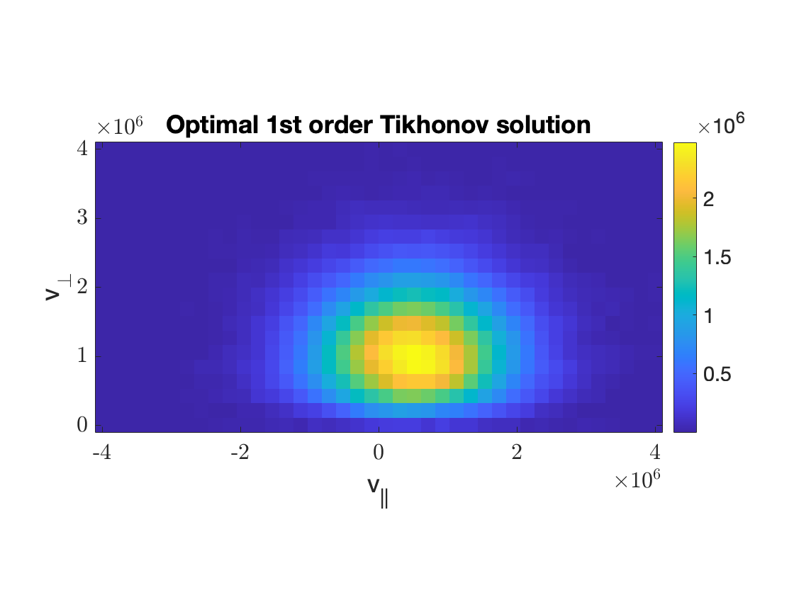
figure
showDistribution(xalpha1(:,idx1),ginfo); title('Optimal 1st order Tikhonov solution')
By executing the code above, we get the following results:
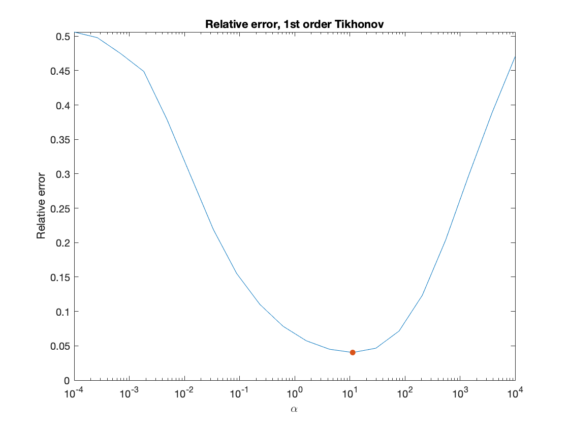
For the 1st order Tikhonov solution, the optimal regularisation parameter \(\alpha = 1.13\cdot10^1\) and minimum relative error of \(0.04030\).
This demo can be found in demos/biMax_recon.m and likewise, if you wish to conduct the same experiment with the slowing-down velocity distribution,
then you can take a look at demos/isoSD_recon.m
Uncertainty Quantification for a bi-Maxwellian distribution
First, the 0th and 1st order Tikhonov example is run just like before. This is such that we have something to compare with.
%% Bi-Maxwellian UQ Example
% This is a demo of Uncertainty Quantification for the bi-Maxwellian
% fast-ion velocity distribution.

clear, clc, close all

[A, b, x, L, ginfo] = biMax();

%Display the true solution
figure
showDistribution(x,ginfo); title('True solution')

%Display nonnegative least-squares solution
figure
showDistribution(TikhNN(A,b,0,[]),ginfo); title('NNLS solution')

%0th order Tikhonov.
disp('Solving 0th order Tikhonov.')
alpha0 = logspace(-15,-8,20);
xalpha0 = TikhNN(A, b, alpha0, []);
[ralpha0, idx0] = relerr(x, xalpha0);
fprintf('Optimal solution: alpha = %.2e, r(alpha) = %.5f\n',alpha0(idx0),ralpha0(idx0))

%1st order Tikhonov.
disp('Solving 1st order Tikhonov.')
alpha1 = logspace(-4,4,20);
xalpha1 = TikhNN(A, b, alpha1, L);
[ralpha1, idx1] = relerr(x, xalpha1);
fprintf('Optimal solution: alpha = %.2e, r(alpha) = %.5f\n',alpha1(idx1),ralpha1(idx1))
Now, we get on to the uncertainty quantification. Here, we do n = 1000 samples and discard 100 as burn-in. In order to make sure that the chains are stationary, this is not enough, but seeing as this is a demonstration it will do.
nsim = 1000; nburnin = 100;

disp('Running Gibbs Sampler with 0th order prior - this might take a while.')
[xsim0, alphasim0, deltasim0, lambdasim0, info0] = NNHGS(A,b,[],nsim);

disp('Running Gibbs Sampler with 1st order prior - this might take a while.')
[xsim1, alphasim1, deltasim1, lambdasim1, info1] = NNHGS(A,b,L,nsim);
Here, xsim contains the samples, alphasim, deltasim and lambdasim contains the \((\alpha, \delta, \lambda)\)-chains, where
\(\alpha := \frac{\delta}{\lambda}\). After this, we can do some convergence analysis and look at the results.
%Convergence plots for 0th order
disp('0th order:')
chain_analysis(deltasim0(nburnin:end),lambdasim0(nburnin:end))

%Convergence plots for 1st order
disp('1st order:')
chain_analysis(deltasim1(nburnin:end),lambdasim1(nburnin:end))

%Plot the regularisation parameters with sample quantiles
%0th order
figure
semilogx(alpha0, ralpha0)
hold on
plot(alpha0(idx0),ralpha0(idx0),'k.', 'MarkerSize', 15) %Optimum
alpha0_mean = mean(alphasim0(nburnin:end)); r0mean = relerr(x,TikhNN(A,b,alpha0_mean));
plot(alpha0_mean, r0mean, 'ro', 'MarkerSize', 10)
qalpha0 = quantile(alphasim0(nburnin:end),[0.025, 0.975]);
errorbar(alpha0_mean, r0mean, ...
         qalpha0(1) - alpha0_mean, ...
         qalpha0(2) - alpha0_mean, ...
         'horizontal','LineWidth',1,'color','r', 'HandleVisibility', 'off')
title('0th order regularisation parameter results')

figure
semilogx(alpha1, ralpha1)
hold on
plot(alpha1(idx1),ralpha1(idx1),'k.', 'MarkerSize', 15) %Optimum
alpha1_mean = mean(alphasim1(nburnin:end)); r1mean = relerr(x,TikhNN(A,b,alpha1_mean,L));
plot(alpha1_mean, r1mean, 'ro', 'MarkerSize', 10)
qalpha1 = quantile(alphasim1(nburnin:end),[0.025, 0.975]);
errorbar(alpha1_mean, r1mean, ...
         qalpha1(1) - alpha1_mean, ...
         qalpha1(2) - alpha1_mean, ...
         'horizontal','LineWidth',1,'color','r', 'HandleVisibility', 'off')
title('1st order regularisation parameter results')

%Plot the credibility bounds
figure
subplot(1,2,1)
showDistribution(mean(xsim0(:,nburnin:end),2),ginfo); title('Sample mean, 0th order prior')
subplot(1,2,2)
showDistribution(cbounds(xsim0(:,nburnin:end)),ginfo); title('95% credibility bounds, 0th order prior')

figure
subplot(1,2,1)
showDistribution(mean(xsim1(:,nburnin:end),2),ginfo); title('Sample mean, 1st order prior')
subplot(1,2,2)
showDistribution(cbounds(xsim1(:,nburnin:end)),ginfo); title('95% credibility bounds, 1st order prior')
The demo can also be found in demos/biMax_UQ.m, and a similar example with the slowing-down distribution can be found in demos/isoSD_UQ.m